Extracting curve coordinates from a bitmap by Mark Seemann
Another example of using Haskell as an ad-hoc scripting language.
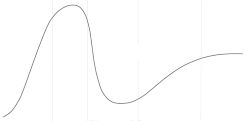
This article is part of a short series titled Trying to fit the hype cycle. In the first article, I outlined what it is that I'm trying to do. In this article, I'll describe how I extract a set of x and y coordinates from this bitmap:

(Actually, this is scaled-down version of the image. The file I work with is a bit larger.)
As I already mentioned in the previous article, these days there are online tools for just about everything. Most likely, there's also an online tool that will take a bitmap like that and return a set of (x, y) coordinates.
Since I'm doing this for the programming exercise, I'm not interested in that. Rather, I'd like to write a little Haskell script to do it for me.
Module and imports #
Yes, I wrote Haskell script. As I've described before, with good type inference, a statically typed language can be as good for scripting as a dynamic one. Just as might be the case with, say, a Python script, you'll be iterating, trying things out until finally the script settles into its final form. What I present here is the result of my exercise. You should imagine that I made lots of mistakes underway, tried things that didn't work, commented out code and print statements, imported modules I eventually didn't need, etc. Just like I imagine you'd also do with a script in a dynamically typed language. At least, that's how I write Python, when I'm forced to do that.
In other words, the following is far from the result of perfect foresight, but rather the equilibrium into which the script settled.
I named the module HypeCoords, because the purpose of it is to extract the (x, y) coordinates from the above Gartner hype cycle image. These are the imports it turned out that I ultimately needed:
module HypeCoords where

import qualified Data.List.NonEmpty as NE
import Data.List.NonEmpty (NonEmpty((:|)))
import Codec.Picture
import Codec.Picture.Types
The Codec.Picture modules come from the JuicyPixels package. This is what enables me to read a .png file and extract the pixels.
Black and white #
If you look at the above bitmap, you may notice that it has some vertical lines in a lighter grey than the curve itself. My first task, then, is to get rid of those. The easiest way to do that is to convert the image to a black-and-white bitmap, with no grey scale.
Since this is a one-off exercise, I could easily do that with a bitmap editor, but on the other hand, I thought that this was a good first task to give myself. After all, I didn't know the JuicyPixels library at all, so this was an opportunity to start with a task just a notch simpler than the one that was my actual goal.
I thought that the easiest way to convert to a black-and-white image would be to turn all pixels white if they are lighter than some threshold, and black otherwise.
A PNG file has more information than I need, so I first converted the image to an 8-bit RGB bitmap. Even though the above image looks as though it's entirely grey scale, each pixel is actually composed of three colours. In order to compare a pixel with a threshold, I needed a single measure of how light or dark it is.
That turned out to be about as simple as it sounds: Just take the average of the three colours. Later, I'd need a function to compute the average for another reason, so I made it a reusable function:
average :: Integral a => NE.NonEmpty a -> a
average nel = sum nel `div` fromIntegral (NE.length nel)
It's a bit odd that the Haskell base library doesn't come with such a function (at least to my knowledge), but anyway, this one is specialized to do integer division. Notice that this function computes only non-exceptional averages, since it requires the input to be a NonEmpty list. No division-by-zero errors here, please!
Once I'd computed a pixel average and compared it to a threshold value, I wanted to replace it with either black or white. In order to make the code more readable I defined two named constants:
black :: PixelRGB8
black = PixelRGB8 minBound minBound minBound
white :: PixelRGB8
white = PixelRGB8 maxBound maxBound maxBound
With that in place, converting to black-and-white is only a few more lines of code:
toBW :: PixelRGB8 -> PixelRGB8
toBW (PixelRGB8 r g b) =
  let threshold = 192 :: Integer
      lum = average (fromIntegral r :| [fromIntegral g, fromIntegral b])
  in if lum <= threshold then black else white
I arrived at the threshold of 192 after a bit of trial-and-error. That's dark enough that the light vertical lines fall to the white side, while the real curve becomes black.
What remained was to glue the parts together to save the black-and-white file:
main :: IO ()
main = do
  readResult <- readImage "hype-cycle-cleaned.png"
  case readResult of
    Left msg -> putStrLn msg
    Right img -> do
      let bwImg = pixelMap toBW $ convertRGB8 img
      writePng "hype-cycle-bw.png" bwImg
The convertRGB8 function comes from JuicyPixels.
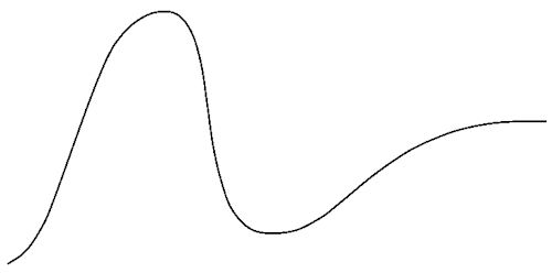
The hype-cycle-bw.png picture unsurprisingly looks like this:

Ultimately, I didn't need the black-and-white bitmap file. I just wrote the script to create the file in order to be able to get some insights into what I was doing. Trust me, I made a lot of stupid mistakes along the way, and among other issues had some 'fun' with integer overflows.
Extracting image coordinates #
Now I had a general feel for how to work with the JuicyPixels library. It still required quite a bit of spelunking through the documentation before I found a useful API to extract all the pixels from a bitmap:
pixelCoordinates :: Pixel a => Image a -> [((Int, Int), a)]
pixelCoordinates = pixelFold (\acc x y px -> ((x,y),px):acc) []
While this is, after all, just a one-liner, I'm surprised that something like this doesn't come in the box. It returns a list of tuples, where the first element contains the pixel coordinates (another tuple), and the second element the pixel information (e.g. the RGB value).
One y value per x value #
There were a few more issues to be addressed. The black curve in the black-and-white bitmap is thicker than a single pixel. This means that for each x value, there will be several black pixels. In order to do linear regression, however, we need a single y value per x value.
One easy way to address that concern is to calculate the average y value for each x value. This may not always be the best choice, but as far as we can see in the above black-and-white image, it doesn't look as though there's any noise left in the picture. This means that we don't have to worry about outliers pulling the average value away from the curve. In other words, finding the average y value is an easy way to get what we need.
averageY :: Integral b => NonEmpty (a, b) -> (a, b)
averageY nel = (fst $ NE.head nel, average $ snd <$> nel)
The averageY function converts a NonEmpty list of tuples to a single tuple. Watch out! The input tuples are not the 'outer' tuples that pixelCoordinates returns, but rather a list of actual pixel coordinates. Each tuple is a set of coordinates, but since the function never manipulates the x coordinate, the type of the first element is just unconstrained a. It can literally be anything, but will, in practice, be an integer.
The assumption is that the input is a small list of coordinates that all share the same x coordinate, such as (42, 99) :| [(42, 100), (42, 102)]. The function simply returns a single tuple that it creates on the fly. For the first element of the return tuple, it picks the head tuple from the input ((42, 99) in the example), and then that tuple's fst element (42). For the second element, the function averages all the snd elements (99, 100, and 102) to get 100 (integer division, you may recall):
ghci> averageY ((42, 99) :| [(42, 100), (42, 102)])
(42,100)
What remains is to glue together the building blocks.
Extracting curve coordinates #
A few more steps were required, but these I just composed in situ. I found no need to define them as individual functions.
The final composition looks like this:
main :: IO ()
main = do
  readResult <- readImage "hype-cycle-cleaned.png"
  case readResult of
    Left msg -> putStrLn msg
    Right img -> do
      let bwImg = pixelMap toBW $ convertRGB8 img
      let blackPixels =
            fst <$> filter ((black ==) . snd) (pixelCoordinates bwImg)
      let h = imageHeight bwImg
      let lineCoords = fmap (h -) . averageY <$> NE.groupAllWith fst blackPixels
      writeFile "coords.txt" $
        unlines $ (\(x,y) -> show x ++ "," ++ show y) <$> lineCoords
The first lines of code, until and including let bwImg, are identical to what you've already seen.
We're only interested in the black pixels, so the main action uses the standard filter function to keep only those that are equal to the black constant value. Once the white pixels are gone, we no longer need the pixel information. The expression that defines the blackPixels value finally (remember, you read Haskell code from right to left) throws away the pixel information by only retaining the fst element. That's the tuple that contains the coordinates. You may want to refer back to the type signature of pixelCoordinates to see what I mean.
The blackPixels value has the type [(Int, Int)].
Two more things need to happen. One is to group the pixels together per x value so that we can use averageY. The other is that we want the coordinates as normal Cartesian coordinates, and right now, they're in screen coordinates.
When working with bitmaps, it's quite common that pixels are measured out from the top left corner, instead of from the bottom left corner. It's not difficult to flip the coordinates, but we need to know the height of the image:
let h = imageHeight bwImg
The imageHeight function is another JuicyPixels function.
Because I sometimes get carried away, I write the code in a 'nice' compact style that could be more readable. I accomplished both of the above remaining tasks with a single line of code:
let lineCoords = fmap (h -) . averageY <$> NE.groupAllWith fst blackPixels
This first groups the coordinates according to x value, so that all coordinates that share an x value are collected in a single NonEmpty list. This means that we can map all of those groups over averageY. Finally, the expression flips from screen coordinates to Cartesian coordinates by subtracting the y coordinate from the height h.
The final writeFile expression writes the coordinates to a text file as comma-separated values. The first ten lines of that file looks like this:
9,13
10,13
11,13
12,14
13,15
14,15
15,16
16,17
17,17
18,18
...
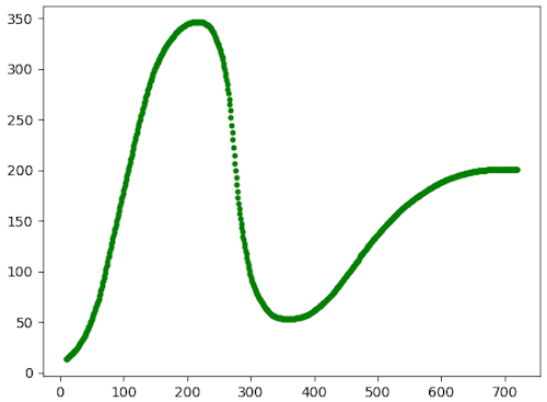
Do these points plot the Gartner hype cycle?
Sanity checking by plotting the coordinates #
To check whether the coordinates look useful, we could plot them. If I wanted to use a few more hours, I could probably figure out how to do that with JuicyPixels as well, but on the other hand, I already know how to do that with Python:
data = numpy.loadtxt('coords.txt', delimiter=',')
x = data[:, 0]
t = data[:, 1]
plt.scatter(x, t, s=10, c='g')
plt.show()
That produces this plot:

LGTM.
Conclusion #
In this article, you've seen how a single Haskell script can extract curve coordinates from a bitmap. The file is 41 lines all in all, including module declaration and white space. This article shows every single line in that file, apart from some blank lines.
I loaded the file into GHCi and ran the main action in order to produce the CSV file.
I did spend a few hours looking around in the JuicyPixels documentation before I'd identified the functions that I needed. All in all I used some hours on this exercise. I didn't keep track of time, but I guess that I used more than three, but probably fewer than six, hours on this.
This was the successful part of the overall exercise. Now onto the fiasco.
